1D Interpolation for B/H, D/H, rb/H

A precursor to this example may be the Dimensioning Rules Example.

Computing Library-like g-Functions

A 7x10 borehole field is created using https://github.com/j-c-cook/Rectangle-Bore-Field-Generator. That layout can be seen in Fig. 3.

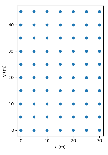
Fig. 3 7x10 borefield layout with 5m uniform spacing

A library like range of g-functions are computed using the following inputs.

The inputs for the B=5m g-functions computed (7x10 borefield)

D (m)	H (m)	rb (m)	B (m)	alpha (m2/s)	nSegments (-)
0.16667	8	0.004	5	1E-06	12
0.25	12	0.006	5	1E-06	12
0.5	24	0.012	5	1E-06	12
1	48	0.024	5	1E-06	12
2	96	0.048	5	1E-06	12
4	192	0.096	5	1E-06	12
8	384	0.192	5	1E-06	12

It should be noted that this corresponds to an rb/H = 0.0005 and D/H = 0.02083.

The g-functions are visualized in Fig. 4

Fig. 4 The g-functions for the 7x10 borefield from Fig. 3

Interpolation for g, D, rb

The table above gives the input values. It can be seen that there are varying D and rb values to keep the D/H ratio and rb/H ratio constant. Therefore, interpolating for a g-function using a B/H ratio will also result in a new rb and D value, though in this case the rb/H and D/H ratios should remain the same even after interpolation.

A B and H value of 8m and 128m are respectively selected for this interpolation example. This corresponds to a B/H of 0.0625, therefore the interpolated value should fall in between the green and red curves in Fig. 4. That corresponds to rb values in a range of 0.024m-0.048m and D values to fall within 1m-2m. The resulting output is the following:

rb = 0.0400     rb/H_eq = 0.0005
D = 1.66667     D/H_eq = 0.02083

The interpolated rb/H and D/H ratios make sense. However, notice that the height is referred to as H_eq or an equivalent height. This is what is returned from calling the interpolation function, gFunctionLibrary.handle_contents.Borefield.g_function_interpolation(). This occurs because the interpolation for a new g-function is a function that is dependent on height.

\[g(ln(t_i/t_s), H_j) = f(H_j)_i\]

Where f could be any method of interpolation: linear, quadratic, cubic, lagrange, etc. This function is originally fit with as many points as there are curves in the library for a particular configuration.

The interpolated g-functions accuracy has already been proven in Dimensioning Rules Example. The interpolated g-function is added and the plot presented in Fig. 5

Fig. 5 The g-functions for the 7x10 borefield and an interpolated g-function for a B/H=0.0625

Source Code

# Jack C. Cook
# Wednesday, February 3, 2021

"""
**interpolation_1D.py**

This example focuses on 1D interpolation over B/H ratios
"""

import gFunctionDatabase as gfl
import matplotlib.pyplot as plt


def main():
    path_to_file: str = 'files/lib/7x10_B_5_nbh_70.json'  # give a path to a file containing computed g-functions
    data: dict = gfl.fileio.js_r(path_to_file)  # if we were to lookup in the library we would have this dict
    # pass the data into the borefield class
    bf = gfl.handle_contents.Borefield(data)
    # visualize this borefield
    fig_1, ax_1 = bf.visualize_borefield()
    fig_1.savefig('7x10_borefield.png')
    plt.close(fig_1)
    # visualize the g-functions
    fig_2, ax_2 = bf.visualize_g_functions()
    fig_2.savefig('7x10_g_functions.png')
    # dont close the figure yet so we can add on the interpolation curve

    # interpolate for a B/H value
    B: float = 8.
    H: float = 128.
    # the default for the kind of interpolation is
    g_interpolated, rb_interpolated, D_interpolated, H_eq = bf.g_function_interpolation(B/H)

    print('The interpolated g-function for a B/H = {}/{}:'.format(B, H))
    print(g_interpolated)
    print('rb = {0:.4f}\trb/H_eq = {1:.4f}'.format(rb_interpolated, rb_interpolated / H_eq))
    print('D = {0:.5f}\tD/H_eq = {1:.5f}'.format(D_interpolated, D_interpolated / H_eq))

    ax_2.plot(bf.log_time, g_interpolated, '^')
    fig_2.savefig('7x10_g_functions_w_interpolated.png')
    plt.close(fig_2)

    # Consider that the borehole radius of the design is different from the interpolated one
    rb_design = 0.075  # borehole radius (m)
    g_function_corrected = gfl.handle_contents.borehole_radius_correction(g_interpolated,
                                                                          rb_interpolated,
                                                                          rb_design)


if __name__ == '__main__':
    main()