Dimensioning Rules Example
A 7x10 borefield is chosen to verify the dimensioning rules of Per Eskilson (1988) [2]. These g-functions have been computed using the methodology of Cimmino and Bernier (2014) [14]. The uniform borehole wall temperature (UBHWT) boundary condition with 12 segments is used, this was the closest when compared to Eskilson. Specifically, this is boundary condition 3 in Cimmino and Bernier (2014). Cimmino went on to implement the g-function calculation in an open source Python package known as pygfunction, which is published on the Python Package Index (PyPI) [12]. Further improvements to the g-function calculation methodology are detailed in Cimmino (2018) [11]. The g-functions in this example are computed using a computationally improved version of Massimo Cimmino’s methodology, which is discussed in Cook and Spitler (2021) [10]. All of the g-functions in this example were computed using the same dimensionless borehole radius, rb/H, and burial depth, D/H, ratios.
Compute g-Functions with varied B/H Ratios
To ensure that the g-function does scale with the dimensionless parameters, g-functions varying different heights are computed for borefields with uniform spacing of 5 and 8 meters. The boundary condition used is uniform borehole wall temperature (UBHWT). There is an additional two g-functions computed with a B/H=0.0625. The following tables display the inputs used:
- Thus, the dimensionless ratios used:
D/H = 0.02083
rb/H = 0.0005
B/H (varies)
- ln(t/ts) - Eskilsons original 27 points
ln(t/ts)_values = [-8.5, -7.8, -7.2, -6.5, -5.9, -5.2, -4.5, -3.963, -3.27, -2.864, -2.577, -2.171,
-1.884, -1.191, -0.497, -0.274, -0.051, 0.196, 0.419, 0.642, 0.873, 1.112, 1.335, 1.679, 2.028, 2.275, 3.003]
The additional g-functions computed with a B/H=0.0625 is given in the following table:
The g-functions from the input tables above are plotted in the Fig. 1. The g-functions computed for the borefield with a uniform spacing, B=5m, are listed in the B/H library legend. This was done because this is like what will be in the library. The g-functions computed using the uniform spacing, B=20m, are listed in the B/H Computed legend. The g-functions which have the same B/H value for the 5m and 20m spacing fields are computed with the same color. There are two additional g-function curves computed for a B/H=0.0625, which will be used as reference for interpolation later on.
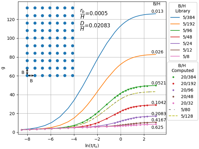
Fig. 1 g-Functions plotted with the same rb/H, D/H and borehole layout (7x10), but with varied B/H values
Additionally, mean percentage errors (computed with gFunctionLibrary.statistics.mpe()) are presented
in the table below.
Interpolation
The g-functions computed with B/H ratios of 0.0625 were computed and are displayed in Fig. 1 to have a reference for checking the accuracy of interpolation using the B/H Library g-functions (all containing a B spacing of 5m). The mean percent errors for different methods of interpolation can be seen in the table below.
An interpolated g-function (using cubic interpolation) is now plotted on an updated Fig. 2.
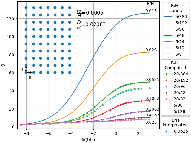
Fig. 2 An interpolated g-function curve of B/H=0.0625 is interpolated for using g-functions computed with a uniform spacing of 5m and ranging heights
Source Code
  1# Jack C. Cook
  2# Tuesday, February 2, 2020
  3
  4"""
  5**dimensioning_rules.py**
  6
  7The following goals will be accomplished in this example:
  8    1) proof that g-functions vary based on ln(t/ts), B/H, D/H, and rb/H
  9    2) proof that interpolation over B/H is accurate
 10"""
 11
 12import gFunctionDatabase as gfl
 13import matplotlib.pyplot as plt
 14from scipy.interpolate import lagrange
 15
 16
 17def main():
 18    # Part 1) Prove that the g-functions vary based on ln(t/ts), B/H, D/H, and rb/H visually and mathematically
 19    # Part A) Collect and plot the g-functions for a library file for a 7x10 borefield where B=5
 20    path_to_lib_files: str = 'files/lib/'  # each of the files in here have g-functions like will be stored in lookup
 21    bf_5m_lib = gfl.handle_contents.Borefield(gfl.fileio.js_r(path_to_lib_files + '7x10_B_5_nbh_70.json'))
 22    fig_1, ax_1 = bf_5m_lib.visualize_g_functions()
 23
 24    # Part B) Collect the g-functions for the library file for a 7x10 borefield where B=20
 25    #         Determine the error when computing B/H values
 26    bf_20m_lib = gfl.handle_contents.Borefield(gfl.fileio.js_r(path_to_lib_files + '7x10_B_20_nbh_70.json'))
 27    # If Eskilson was right, and the dimensioning rules are accurate, then the following mean percent errors will be ~0
 28    keys_5m = list(reversed(list(bf_5m_lib.g.keys())))
 29    keys_5m = keys_5m[2:]
 30    print('The heights that will be used in the from the 5m library file:')
 31    print(keys_5m)
 32    print('The heights that will be used in the from the 20m library file:')
 33    keys_20m = list(reversed(list(bf_20m_lib.g.keys())))
 34    print(keys_20m)
 35
 36    mean_percent_errors = []
 37    for i in range(len(keys_5m)):
 38        mean_percent_error = gfl.statistics.mpe(bf_5m_lib.g[keys_5m[i]], bf_20m_lib.g[keys_20m[i]])
 39        mean_percent_errors.append(mean_percent_error)
 40    print('Mean percent errors between g-functions')
 41    print(mean_percent_errors)
 42
 43    # Part C) Plot the g-functions for the B=20 7x10 borefield
 44    lines = []
 45    for i, key in enumerate(keys_20m):
 46        line, = ax_1.plot(bf_20m_lib.log_time, bf_20m_lib.g[key], marker='o', ls='None', color='C' + str(i + 2),
 47                          markersize=3,
 48                          label=str(int(bf_20m_lib.B)) + '/' + str(key))
 49        lines.append(line)
 50
 51    # Part D) Plot a B/H of 0.0625 which is 8/128 and 5/8
 52    path_to_computed = 'files/computed/'
 53    bf_computed_5m = gfl.handle_contents.Borefield(gfl.fileio.js_r(path_to_computed + '7x10_B_5_nbh_70.json'))
 54    bf_computed_8m = gfl.handle_contents.Borefield(gfl.fileio.js_r(path_to_computed + '7x10_B_8_nbh_70.json'))
 55    line_7, = ax_1.plot(bf_computed_5m.log_time, bf_computed_5m.g[80], ls=(0, (3, 5, 1, 5)),
 56                        label=str(int(bf_computed_5m.B)) + '/' + str(80), zorder=2)
 57    line_8, = ax_1.plot(bf_computed_5m.log_time, bf_computed_8m.g[128], ls='dashed',
 58                        label=str(int(bf_computed_5m.B)) + '/' + str(128), zorder=1)
 59    lines.append(line_7)
 60    lines.append(line_8)
 61    second_legend = fig_1.legend(handles=lines,
 62                                 title='B/H'.rjust(8) + '\nComputed', bbox_to_anchor=(1.005, 0.6))
 63    fig_1.gca().add_artist(second_legend)
 64
 65    # Part E) Annotate the plot with the borehole layout and the D/H, rb/H
 66    # add in a sub axes plot with the borehole layout
 67    sub_axes = plt.axes([.0, .47, .5, .5])
 68    x, y = list(zip(*bf_5m_lib.bore_locations))
 69    sub_axes.scatter(x, y)
 70    sub_axes.set_aspect('equal')
 71    sub_axes.axis('off')
 72    # annotate the layout with B spacings
 73    sub_axes.annotate(text='', xy=(0, 0), xytext=(5, 0), arrowprops=dict(arrowstyle='<->'))
 74    sub_axes.annotate(text='', xy=(0, 0), xytext=(0, 5), arrowprops=dict(arrowstyle='<->'))
 75    ax_1.text(-7.8, 53, 'B')
 76    ax_1.text(-8.5, 62, 'B')
 77    # add in text for D/H and rb/H
 78    ax_1.text(-3.5, 124, '$\dfrac{r_b}{H}$=0.0005', fontsize=12)
 79    ax_1.text(-3.5, 111, '$\dfrac{D}{H}$=0.02083', fontsize=12)
 80
 81    fig_1.savefig('dimensioning_rules_figure_01.png')
 82
 83    # Part F) Interpolate for a B/H = 0.0625
 84    B: float = 8.
 85    H: float = 128.
 86    B_over_H: float = B / H
 87    interpolation_kinds = ['linear', 'quadratic', 'cubic', 'lagrange']
 88    g_functions = []
 89    for kind in interpolation_kinds:
 90        g_function, _, _, _ = bf_5m_lib.g_function_interpolation(B_over_H, kind=kind)
 91        bf_5m_lib.interpolation_table = {}  # this needs reset to recompute the table with a new kind
 92        g_functions.append(g_function)
 93    mean_percentage_errors = []
 94    for i in range(len(g_functions)):
 95        MPE = gfl.statistics.mpe(bf_computed_5m.g[80], g_functions[i])
 96        mean_percentage_errors.append(MPE)
 97    print('The errors associated with different interpolation methods:')
 98    for i in range(len(interpolation_kinds)):
 99        print('\t{0}:\t{1:.2f}%'.format(interpolation_kinds[i], mean_percentage_errors[i]))
100    mean_percent_errors_abs = list(map(abs, mean_percentage_errors))
101    idx = mean_percent_errors_abs.index(min(mean_percent_errors_abs))
102    print('{} interpolation is the most accurate'.format(interpolation_kinds[idx]))
103    g_function = g_functions[idx]
104    line_10, = ax_1.plot(bf_5m_lib.log_time, g_function, marker='^', zorder=0, color='C9', markersize=5, ls='None',
105                         label='0.0625')
106
107    third_legend = fig_1.legend(handles=[line_10],
108                                title='B/H'.rjust(10) + '\nInterpolated', bbox_to_anchor=(1.005, 0.2))
109    fig_1.gca().add_artist(third_legend)
110
111    fig_1.savefig('dimensioning_rules_figure_02.png')
112    plt.close(fig_1)
113
114
115if __name__ == '__main__':
116    main()